Python-Data-Analysis(python 数据分析)

字数统计: 2.4k阅读时长: 11 min

 2019/10/17 

第二章ipython jupyter的特性
- 魔术命令
  - %timeit 测试执行时间
  - %debug
  - %pwd 输出当前目录
  - %whos 显示空间变量
  - %run 运行代码
  - %reset 删除所有空间变量和名字
  - %pdb 出现异常自动进入调试模式
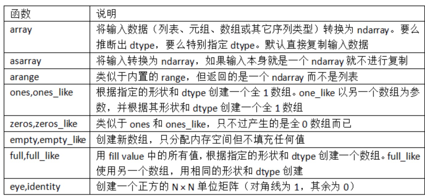
第四章 Numpy基础
- ndarray 多维数组对象
  - dtype 数据类型
  - shape 各维度大小
- 切片索引会直接改变原有结果(按引用传递的概念)
- 花式索引 Fancy indexing
  -它指的是利用整数数组进行索引。
  -花式索引跟切片不一样，它总是将数据复制到新数组中
- 通用函数
  - np.maximum(ndarray1,ndarray2)计算了x和y中元素级别最大的元素。
  - np.sqrt(ndarray) 开平方
  - np.modf(ndarray) 拆分浮点数
- 数学和统计方法
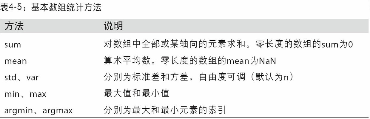
  - np.mean(ndarray,axis=0/1) 计算平均值/指定轴 0:x/1:y
  - np.quantile(0.4) 计算40%的分位数
  - np.cumsum(ndarray, axis=0/1) 累计和
  - np.cumprod(ndarray, axis=0/1) 累计积
- 线性代数
- 随机函数
  - np.random
    - random.randn(line_Num, column_num) : 从标准正态分布中返回一个或多个样本值。
    - random.rand() : 随机样本位于[0, 1)中
    - random.randint(low=10,high=100, size=(5,5,5)) : 返回555 维鉴于10-100的ndarray
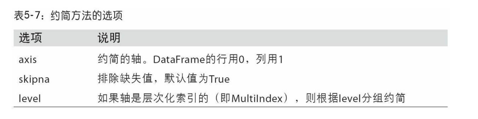
第五章:pandas入门
- 数据结构
  - DataFrame: 表格型数据结构,包含一组有序的列
    - 为了更准确选择数据，请使用loc（标签）或iloc（整数)
    - 汇总和计算描述统计函数 df.sum(axis=1)求和(axis=0列求和 axis=1行求和)
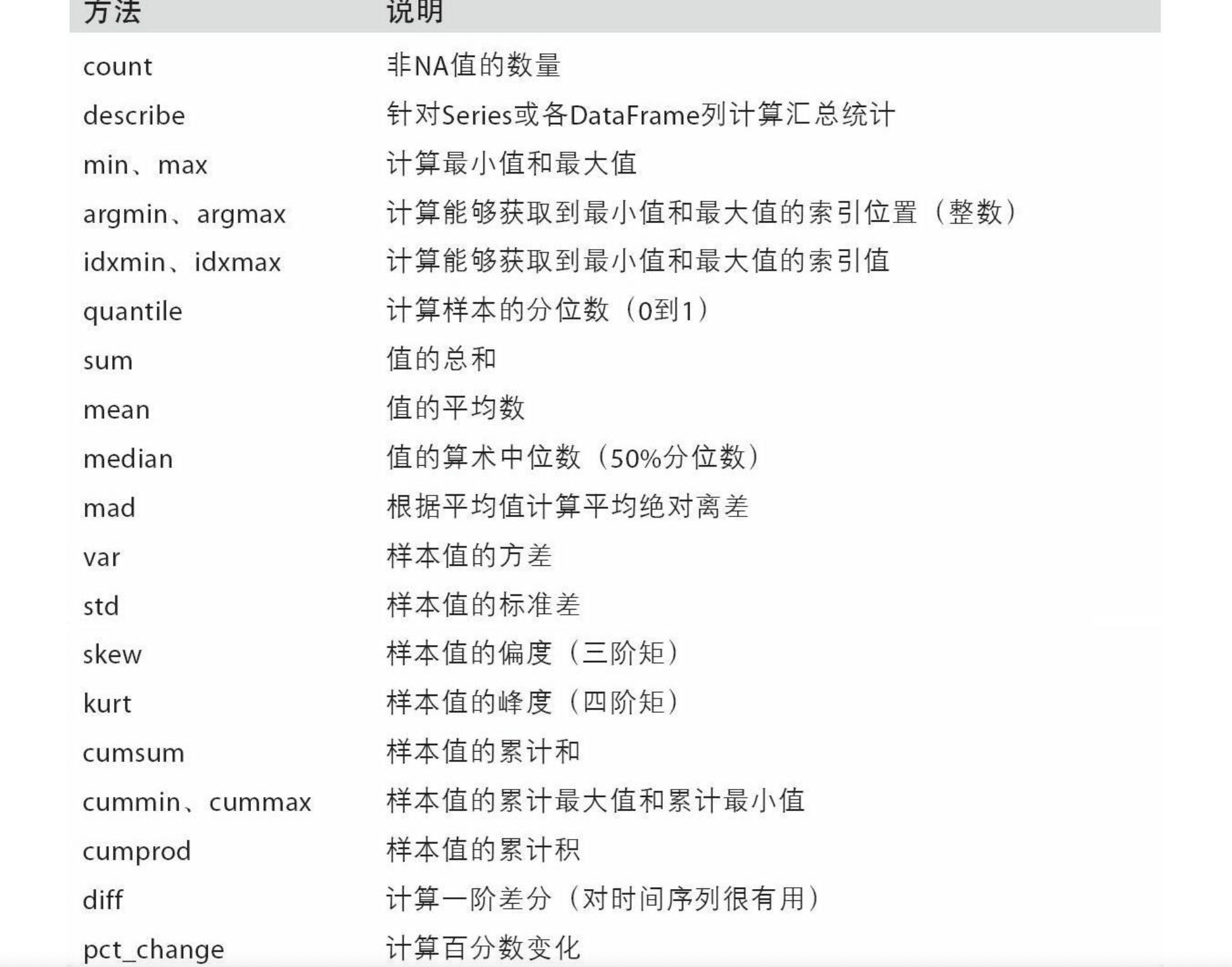
    - 求变化率 df.pct_change()
    - dataFrame[[column1,column2]] DataFrame
    - dataFrame[column1] Series
第六章: 数据加载,存储/文件格式
- pandas 加载
  - pd函数 pandas - tip
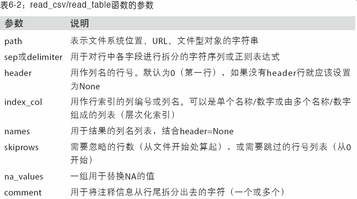
    (evernote:///view/498226/s4/7cdcc8cc-4027-4507-9010-3c4fbc0f8f34/7cdcc8cc-4027-4507-9010-3c4fbc0f8f34/)
  - pd.read_csv(file,na_values={‘message’: [‘foo’, ‘NA’], ‘something’: [‘two’]}) : 默认读取,分割的csv信息为DataFrame格式, message列的foo/NA 都按NaN处理
- WEB API 调用交互
  - pd.DataFrame(requests.get(url).json(),columns=[a1,b2,c3] ) //读取接口返回json中的指定columns字段,生成表格数据结构
第七章: 数据清洗和准备
- 填充
  - df.fillna(0) , 以0替换na
  - df.fillna(method=’ffill/bfill’,axis=0/1) , 以之前/后(行/列)的非缺失值作为替换Nan的数据
  - df.fillna(df.mean()) , 按指定列平均值替换Nan数据
  - df.drop_duplicates([‘k1],keep=’last’), 丢弃k1列重复的数据,并保留最后一个
- 替换
  - df.replace({-999:np.nan,-1000:0}) 将数据中的-999替换成为nan,-1000替换成为0
- axis indexes rename(轴索引重命名)
  - df.rename(index={‘a’:’a-replace’,’b’:’b-replace’},columns={‘ac’:’ac-replace’} , inplace=True)重命名各轴的标签名, 更改原数据
  - df.index.map(lambda x: x[:4].upper()) 改index的表情名, 取字符串前4位,并全部转化为大写
- Discretization and Binning(离散化/面元划分)
  - pd.cut(data, 4, precision=2) 小数位2precision data.均分4分
  - pd.cut(data, bins) 按照bins间隔换分data
  - pd.qcut(data, bins) 自定义的bins
- Detecting and Filtering Outliers(检测过滤异常)
  - data[(np.abs(data) > 3).any(1)] 过滤
  - np.sign(data) 根据数据的值是正还是负，np.sign(data)可以生成1和-1：\\
  - 的
- 哑变量(虚拟变量)? 离散特征量化手段哑变量
  - pd.get_dummies(df[‘column’],prefix=’xxx’), 把df[‘column’]列转换为哑变量矩阵,并且以prefix为前缀
第八章: 数据规整:聚合,合并和重塑 @todo
- Hierarchical Indexing(层次化索引)
  - f

第九章:绘图/可视化

fig = matplotlib.pyplot.figure() //初始化画布
fig.add_subplot(2,2,1) 构建2*2 图像,并选中第1个.
ax = fig.plot(x, y, g–) / fig.plot(x, y , linestyle=’–’, color=’g’) ,绘制绿色虚线连续线图
ax.set_xticklabels([‘one’],rotation=30,fontsize=’larger’) 设置subplot 的x label 倾斜30°, 大字体
ax .legend(loc=’best’,title=’hell’) 设置图标右上角比例提示

批量设置属性

props1 = {
'title' : 'My First Matplotlib Plot!', //设置标题
'xlabel': 'Stages', //设置x label
'ylabel': 'rate',
'xlim':[2,8], //设置x起始值,结束值
'ylim':[-1,1]
}
axs[1].set(**props1)

plt.savefig(‘figpath.png’,dpi=400,bbox_inches=’tight’) 当前目录保存为400像素最小白边的png图片
dataFrame.plot(kind=’box’,title=’box’,alpha=0.7, color=’k’) // 箱图,透明度0.7, k颜色
dataFrame.plot(kind=’bar’,title=’bar’) //祖壮图

dataFrame.plot(kind=’line’,title=’line’) //线图

python	pandas.DataFrame基本函数
查看数据	.head() .tail() .shape .describe()
矩阵运算	.add() .sub() .mul() .div() .divmod() .combine()
矩阵比较	.eq() .ne() .lt() .gt() .le() .ge()
数据框连接	.align() .merge() .join() .concatenate()
设置行名列名	.column .reindex() .reindex_like()
列操作	.drop() .insert() .assign()
数据类型	.dtypes .get_dtype_counts() .astype() .to_numeric()… .select_dtypes()
数据运算	.pipe() .apply() .applymap()
统计运算	.cut() .qcut() .idxmin() .idxmax() .value_counts() .sum()…
排序	.sort_index() .sort_values() .nsmallest() .nlargest()
其他	.dt Iteration .copy() .info()

直方图(histogram)/密度图(kde)
- f

第十章数据聚合与分组运算
- split-apply-combine(拆分-应用-合并)
- 随机采样/排列
  - 的
- 分组加权平均数和相关系数
  - v
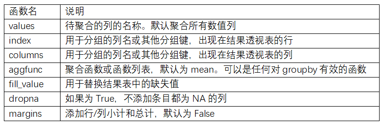
- df.pivot_table() Pivot Tables: 透视表的参数说明请参见表10-2。
- df.Crosstab() Cross-Tabulations:交叉表
  1
  pd.crosstab(data.Nationality, data.Handedness, margins=True) === pd.pivot_table(data=data,index=['Nationality'], columns=['Handedness'],aggfunc='count',margins=True, margins_name='综合')

第十一章时间序列

日期转换: df.to_period(‘M’) : 转换日期格式为每月 2012-01-01 –> 2012-01

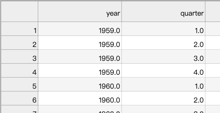
数组生成periodIndex:

1 2	>> pd.PeriodIndex(year=data.year, quarter=data.quarter, freq='Q-DEC') >>

freq:

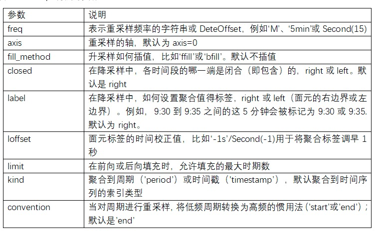
降采样:
`resaTs = ts.resample(‘5min’, closed=’right’,

label='right', loffset='-1s').sum() `:重新按照5min间隔, 右封闭, 右lable -1s 为key名, 样本和

1
2
3
4
5
6
7
8
9
10
11
12
13
ts: 
2000-01-01 00:00:00     0
2000-01-01 00:01:00     1
2000-01-01 00:02:00     2
2000-01-01 00:03:00     3
2000-01-01 00:04:00     4
2000-01-01 00:05:00     5
...
resaTs:
1999-12-31 23:59:59     0
2000-01-01 00:04:59    15
2000-01-01 00:09:59    40
2000-01-01 00:14:59    11

OHLC重采样(resampling): 融领域中有一种无所不在的时间序列聚合方式，即计算各面元的四个值：第一个值（open，开盘）、最后一个值（close，收盘）、最大值（high，最高）以及最小值（low，最低）
- df.resample(rule=’M’, kind=).
  - 升采样/插值
    df.resample(‘D’).asfreq() : 强制升采样
  Year Colorado Texas
  
  2000-01-05 0.746433 2.224660
  
  2000-01-12 -0.679400 0.727369
  
  ===>
  
  Year Colorado Texas
  
  2000-01-05 0.746433 2.224660
  
  2000-01-06 Nan Nan
  
  …
  
  Year Colorado Texas
  
  2000-01-12 -0.679400 0.727369
指数加权函数
- 否

Year	Colorado	Texas
2000-01-05	0.746433	2.224660
2000-01-12	-0.679400	0.727369

Year	Colorado	Texas
2000-01-05	0.746433	2.224660
2000-01-06	Nan	Nan
…

Year	Colorado	Texas
2000-01-12	-0.679400	0.727369

第十二章 pandas高级应用

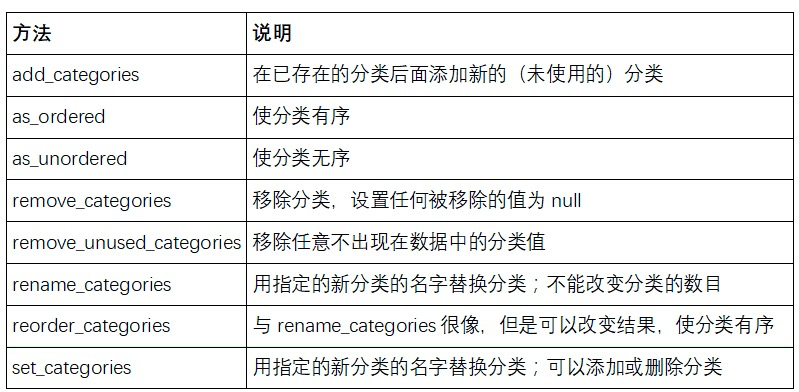
seriesData.take(seriesData) : 用整形表示类别的方法 : 分类

>> values = d.Series([0, 1, 0, 0] * 2)
>> dim = d.Series(['apple','orange'])
>> dim.take(values)
>> 
0     apple
1    orange
0     apple
0     apple
0     apple
1    orange
0     apple
0     apple

SeriseData.astype(‘category’).act.xxxx
pd.get_dummies(pd.
df.groupby(‘key’).value.transform(lambda x: x.mean()) 求取与df同等格式的平均值DataFrame

链式编程

df2 = df.assign(k=v) 
==等价于= 
df2 == df.copy()
df2['k'] = v

# =========> 原始
df = load_data()
df2 = df[df['col2'] < 0]
df2['col1_demeaned'] = df2['col1'] - df2['col1'].mean()
result = df2.groupby('key').col1_demeaned.std()

# =========> 转化过程
# Usual non-functional way
df2 = df.copy()
df2['k'] = v

# Functional assign way
df2 = df.assign(k=v)
result = (df2.assign(col1_demeaned=df2.col1 - df2.col2.mean())
          .groupby('key')
          .col1_demeaned.std())
df = load_data()
df2 = df[df['col2'] < 0]
df = (load_data()
      [lambda x: x['col2'] < 0])

#=========> 最终
result = (load_data()
          [lambda x: x.col2 < 0]
          .assign(col1_demeaned=lambda x: x.col1 - x.col1.mean())
          .groupby('key')
          .col1_demeaned.std())

第十三章 python 建模库

np.ndarray 是 pandas与其他分析库的数据中介桥梁
dataFrame.value => np.ndarray

变量的虚化,产生虚拟变量

 # 为categroy 变量,创建虚变量,并替换自己
 >>> data = pd.DataFrame({
 'x0': [1, 2, 3, 4, 5],
 'x1': [0.01, -0.01, 0.25, -4.1, 0.],
 'y': [-1.5, 0., 3.6, 1.3, -2.]})
 
 >>> data['category'] = pd.Categorical(['a', 'b', 'a', 'a', 'b'],
                               categories=['a', 'b'])
 >>> data => 
 x0	x1	y	category
 0	1	0.01	-1.5	a
 1	2	-0.01	0.0	b
 2	3	0.25	3.6	a
 3	4	-4.10	1.3	a
 4	5	0.00	-2.0	b
 
>>>  #说明: type(data.y.values) ==> numpy.ndarray
 # type(data.category.values) ==> pandas.core.categorical.Categorical
 
 >>> dummies = pd.get_dummies(data.category, prefix='category')
 data.drop('category', axis=1).join(dummies)
 
>>> result ==> 
 	x0	x1	y	category_a	category_b
 0	1	0.01	-1.5	1	0
 1	2	-0.01	0.0	0	1
 2	3	0.25	3.6	1	0
 3	4	-4.10	1.3	1	0
 4	5	0.00	-2.0	0	1

Patsy(库)线性模型描述(创建数据矩阵)

 >>> df = pd.DataFrame({
     'x0':[1,2,3],
     'x1': [0.1,0.1,0.25],
     'y' : [-1.5, 3.6, -2.]
 })
 >>> y, X = patsy.dmatrices('y ~ x0 + x1', data)
>>>  y
 DesignMatrix with shape (5, 1)
          y
       -1.5
        0.0
        3.6
        1.3
       -2.0
       Terms:
         'y' (column 0)
 >>> X 
 DesignMatrix with shape (5, 3)
   Intercept  x0     x1
           1   1   0.01
           1   2  -0.01
           1   3   0.25
           1   4  -4.10
           1   5   0.00
   Terms:
     'Intercept' (column 0)
     'x0' (column 1)
     'x1' (column 2)

用Patsy公式进行数据转换

#使用样本的design规则, 格式化新数据
>>> new_data = pd.DataFrame({
    'x0': [6, 7, 8, 9],
    'x1': [3.1, -0.5, 0, 2.3],
    'y': [1, 2, 3, 4]})
>>> patsy.build_design_matrices([X.design_info], new_data)
>>> y, X = patsy.dmatrices('y ~ I(x0 + x1)', data) # 按照x0+x1的结果构建矩阵